Getting started
In this tutorial we will read HARPS spectra, extract and plot three activity indicators and radial velocity for the star HD41248.
Start by importing and initializing ACTIN
[1]:
%matplotlib inline

from actin2 import ACTIN
actin = ACTIN()
Get the HARPS 1D fits files of the star HD41248 from the test folder
[2]:
import glob, os
files = glob.glob(os.path.join(os.pardir, "actin2/test/HARPS/HD41248", "*_s1d_A.fits"))
files
[2]:
['../actin2/test/HARPS/HD41248/HARPS.2014-01-24T01:18:06.472_s1d_A.fits',
 '../actin2/test/HARPS/HD41248/HARPS.2014-01-16T06:24:23.418_s1d_A.fits',
 '../actin2/test/HARPS/HD41248/HARPS.2014-01-24T04:17:29.213_s1d_A.fits',
 '../actin2/test/HARPS/HD41248/HARPS.2014-01-21T05:33:32.740_s1d_A.fits',
 '../actin2/test/HARPS/HD41248/HARPS.2014-01-21T03:16:16.891_s1d_A.fits',
 '../actin2/test/HARPS/HD41248/HARPS.2014-01-16T05:37:46.157_s1d_A.fits']
Check which indices come pre-installed. We start by looking at the full indices table:
[3]:
actin.IndTable().table
[3]:
| ind_id | ind_var | ln_id | ln_c | ln_ctr | ln_win | bandtype | |
|---|---|---|---|---|---|---|---|
| 0 | I_CaII | L1 | CaIIK | 1.0 | 3933.664 | 1.09 | tri |
| 1 | I_CaII | L2 | CaIIH | 1.0 | 3968.470 | 1.09 | tri |
| 2 | I_CaII | R1 | CaIIR1 | 1.0 | 3901.070 | 20.00 | sq |
| 3 | I_CaII | R2 | CaIIR2 | 1.0 | 4001.070 | 20.00 | sq |
| 4 | I_NaI | L1 | NaID1 | 1.0 | 5895.920 | 0.50 | sq |
| 5 | I_NaI | L2 | NaID2 | 1.0 | 5889.950 | 0.50 | sq |
| 6 | I_NaI | R1 | NaIR1 | 1.0 | 5805.000 | 10.00 | sq |
| 7 | I_NaI | R2 | NaIR2 | 1.0 | 6097.000 | 20.00 | sq |
| 8 | I_Ha16 | L1 | Ha16 | 1.0 | 6562.808 | 1.60 | sq |
| 9 | I_Ha16 | R1 | HaR1 | 1.0 | 6550.870 | 10.75 | sq |
| 10 | I_Ha16 | R2 | HaR2 | 1.0 | 6580.310 | 8.75 | sq |
| 11 | I_Ha06 | L1 | Ha06 | 1.0 | 6562.808 | 0.60 | sq |
| 12 | I_Ha06 | R1 | HaR1 | 1.0 | 6550.870 | 10.75 | sq |
| 13 | I_Ha06 | R2 | HaR2 | 1.0 | 6580.310 | 8.75 | sq |
| 14 | I_HeI | L1 | HeI | 1.0 | 5875.620 | 0.40 | sq |
| 15 | I_HeI | R1 | HeIR1 | 1.0 | 5869.000 | 5.00 | sq |
| 16 | I_HeI | R2 | HeIR2 | 1.0 | 5881.000 | 5.00 | sq |
| 17 | I_CaI | L1 | CaI | 1.0 | 6572.795 | 0.34 | tri |
| 18 | I_CaI | R1 | HaR1 | 1.0 | 6550.870 | 10.75 | sq |
| 19 | I_CaI | R2 | HaR2 | 1.0 | 6580.310 | 8.75 | sq |
The available indices are:
[4]:
actin.IndTable().indices
[4]:
['I_CaI', 'I_CaII', 'I_Ha06', 'I_Ha16', 'I_HeI', 'I_NaI']
We are going to calculate the indices based on the CaII H&K, H\(\alpha\) (using 0.6 ang central band) and NaI D2 lines using the respective index ID as in ind_id:
[5]:
indices = ['I_CaII', 'I_Ha06', 'I_NaI']
Now calculate the indices for the loaded files. The results will be stored in a pandas DataFrame.
[6]:
df = actin.run(files, indices)
100%|██████████| 6/6 [00:02<00:00, 2.94it/s]
See the results headers
[7]:
df.keys()
[7]:
Index(['obj', 'instr', 'date_obs', 'bjd', 'drs', 'exptime', 'ra', 'dec',
       'snr7', 'snr50', 'prog_id', 'pi_coi', 'cal_th_err', 'berv', 'spec_rv',
       'snr_med', 'ftype', 'rv_flg', 'rv', 'dvrms', 'ccf_noise', 'fwhm',
       'cont', 'ccf_mask', 'drift_noise', 'drift_rv', 'rv_wave_corr', 'rv_err',
       'spec_flg', 'file', 'I_CaII', 'I_CaII_err', 'I_CaII_Rneg', 'I_Ha06',
       'I_Ha06_err', 'I_Ha06_Rneg', 'I_NaI', 'I_NaI_err', 'I_NaI_Rneg',
       'actin_ver'],
      dtype='object')
and the full table
[8]:
df
[8]:
| obj | instr | date_obs | bjd | drs | exptime | ra | dec | snr7 | snr50 | ... | I_CaII | I_CaII_err | I_CaII_Rneg | I_Ha06 | I_Ha06_err | I_Ha06_Rneg | I_NaI | I_NaI_err | I_NaI_Rneg | actin_ver | |
|---|---|---|---|---|---|---|---|---|---|---|---|---|---|---|---|---|---|---|---|---|---|
| 0 | HD41248 | HARPS | 2014-01-16T05:37:46.156 | 2.456674e+06 | HARPS_3.7 | 600.0005 | 90.136003 | -56.16330 | 12.0 | 55.6 | ... | 0.126963 | 0.001206 | 0.002865 | 0.107759 | 0.000652 | 0.0 | 0.358022 | 0.001249 | 0.0 | 2.0 beta 8 |
| 1 | HD41248 | HARPS | 2014-01-16T06:24:23.418 | 2.456674e+06 | HARPS_3.7 | 600.0007 | 90.139297 | -56.16415 | 12.4 | 55.6 | ... | 0.138301 | 0.001236 | 0.001154 | 0.105833 | 0.000653 | 0.0 | 0.356299 | 0.001252 | 0.0 | 2.0 beta 8 |
| 2 | HD41248 | HARPS | 2014-01-21T03:16:16.890 | 2.456679e+06 | HARPS_3.7 | 900.0010 | 90.138288 | -56.16339 | 26.5 | 101.3 | ... | 0.145480 | 0.000697 | 0.000000 | 0.105242 | 0.000374 | 0.0 | 0.357987 | 0.000708 | 0.0 | 2.0 beta 8 |
| 3 | HD41248 | HARPS | 2014-01-21T05:33:32.739 | 2.456679e+06 | HARPS_3.7 | 900.0005 | 90.135625 | -56.16338 | 24.6 | 98.0 | ... | 0.141643 | 0.000732 | 0.000000 | 0.105055 | 0.000386 | 0.0 | 0.357836 | 0.000731 | 0.0 | 2.0 beta 8 |
| 4 | HD41248 | HARPS | 2014-01-24T01:18:06.471 | 2.456682e+06 | HARPS_3.7 | 600.0018 | 90.136782 | -56.16351 | 15.7 | 67.6 | ... | 0.139618 | 0.001047 | 0.000194 | 0.106154 | 0.000542 | 0.0 | 0.356930 | 0.001037 | 0.0 | 2.0 beta 8 |
| 5 | HD41248 | HARPS | 2014-01-24T04:17:29.213 | 2.456682e+06 | HARPS_3.7 | 600.0014 | 90.138346 | -56.16322 | 16.4 | 68.2 | ... | 0.137774 | 0.001003 | 0.000208 | 0.107019 | 0.000551 | 0.0 | 0.357135 | 0.001038 | 0.0 | 2.0 beta 8 |
6 rows × 40 columns
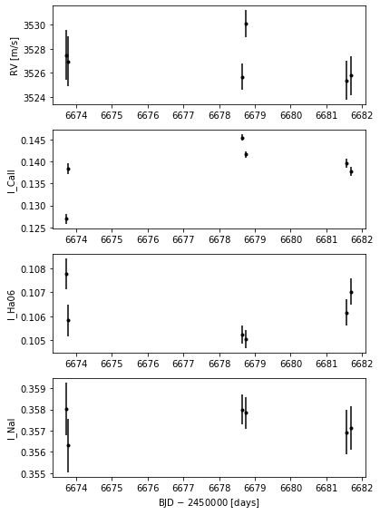
and plot the results
[9]:
import matplotlib.pylab as plt

plt.figure(figsize=(6, (len(indices)+1)*2))

plt.subplot(len(indices)+1, 1, 1)
plt.ylabel("RV [m/s]")
plt.errorbar(df.bjd - 2450000, df.rv, df.rv_err, fmt='k.')

for i, index in enumerate(indices):
    plt.subplot(len(indices)+1, 1, i+2)
    plt.ylabel(index)
    plt.errorbar(df.bjd - 2450000, df[index], df[index + "_err"], fmt='k.')
plt.xlabel("BJD $-$ 2450000 [days]")
plt.tight_layout()