The indices table

All the indices and respective spectral lines information is stored in the indices table file, actin_table.csv.

The table can be accessed from ACTIN via:

from actin2 import ACTIN
actin = ACTIN()

actin.IndTable().table

	ind_id	ind_var	ln_id	ln_c	ln_ctr	ln_win	bandtype
0	I_CaII	L1	CaIIK	1.0	3933.664	1.09	tri
1	I_CaII	L2	CaIIH	1.0	3968.470	1.09	tri
2	I_CaII	R1	CaIIR1	1.0	3901.070	20.00	sq
3	I_CaII	R2	CaIIR2	1.0	4001.070	20.00	sq
4	I_NaI	L1	NaID1	1.0	5895.920	0.50	sq
5	I_NaI	L2	NaID2	1.0	5889.950	0.50	sq
6	I_NaI	R1	NaIR1	1.0	5805.000	10.00	sq
7	I_NaI	R2	NaIR2	1.0	6097.000	20.00	sq
8	I_Ha16	L1	Ha16	1.0	6562.808	1.60	sq
9	I_Ha16	R1	HaR1	1.0	6550.870	10.75	sq
10	I_Ha16	R2	HaR2	1.0	6580.310	8.75	sq
11	I_Ha06	L1	Ha06	1.0	6562.808	0.60	sq
12	I_Ha06	R1	HaR1	1.0	6550.870	10.75	sq
13	I_Ha06	R2	HaR2	1.0	6580.310	8.75	sq
14	I_HeI	L1	HeI	1.0	5875.620	0.40	sq
15	I_HeI	R1	HeIR1	1.0	5869.000	5.00	sq
16	I_HeI	R2	HeIR2	1.0	5881.000	5.00	sq
17	I_CaI	L1	CaI	1.0	6572.795	0.34	tri
18	I_CaI	R1	HaR1	1.0	6550.870	10.75	sq
19	I_CaI	R2	HaR2	1.0	6580.310	8.75	sq

The columns of the table are following:

• ind_id: The index identification. For the spectral lines to be assigned to an index, their ind_id entries must have the same index ID.

• ind_var: The identification of the line in the index equation: L1, L2, etc, for activity lines (numerator); R1, R2, etc, for reference lines (denominator)

• ln_id: The spectral line identification.

• ln_c: Constant to be multiplied to the flux in each line.

• ln_ctr: Line centre (in angstroms).

• ln_win: Bandwidth (in angstroms).

• bandtype: Function used to integrate the flux in the bandpass: sq for square; tri for triangular. If using the triangular bandpass, ln_win is the full-width-half-maximum of the triangle.

To check the available indices use:

actin.IndTable().indices

['I_CaI', 'I_CaII', 'I_Ha06', 'I_Ha16', 'I_HeI', 'I_NaI']

All indices IDs use the prefix I_ to identify the name as an index as opposed to the line ID.

Each index should be associated with its required lines, even if reusing the same lines for different indices (e.g. the HaR1 lines for I_Ha06 and I_Ha16 appear repeated in the table).

Adding new indices

To add a new index, you will need at least an activity sensitive line (with ind_var of L1) and a reference line (ind_var of R1), although it is recommended to have two reference lines, at each side of the activity line in the continuum.

As an example let’s make a new index based on the FeII line at \(\lambda\) 6149.24 (not an activity sensitive index!):

ind_tab = actin.IndTable()

FeII = dict(
    ind_id = "I_FeII",
    ind_var = "L1",
    ln_id = "FeII",
    ln_c = 1,
    ln_ctr = 6149.24,
    ln_win = 0.2,
    bandtype = "sq"
)

FeIIR1 = dict(
    ind_id = "I_FeII",
    ind_var = "R1",
    ln_id = "FeIIR1",
    ln_c = 1,
    ln_ctr = 6146.97,
    ln_win = 1,
    bandtype = "sq"
)

FeIIR2 = dict(
    ind_id = "I_FeII",
    ind_var = "R2",
    ln_id = "FeIIR2",
    ln_c = 1,
    ln_ctr = 6152.42,
    ln_win = 1,
    bandtype = "sq"
)

ind_tab.add_line(**FeII)
ind_tab.add_line(**FeIIR1)
ind_tab.add_line(**FeIIR2)

Now check the new table:

ind_tab.table

	ind_id	ind_var	ln_id	ln_c	ln_ctr	ln_win	bandtype
0	I_CaII	L1	CaIIK	1.0	3933.664	1.09	tri
1	I_CaII	L2	CaIIH	1.0	3968.470	1.09	tri
2	I_CaII	R1	CaIIR1	1.0	3901.070	20.00	sq
3	I_CaII	R2	CaIIR2	1.0	4001.070	20.00	sq
4	I_NaI	L1	NaID1	1.0	5895.920	0.50	sq
5	I_NaI	L2	NaID2	1.0	5889.950	0.50	sq
6	I_NaI	R1	NaIR1	1.0	5805.000	10.00	sq
7	I_NaI	R2	NaIR2	1.0	6097.000	20.00	sq
8	I_Ha16	L1	Ha16	1.0	6562.808	1.60	sq
9	I_Ha16	R1	HaR1	1.0	6550.870	10.75	sq
10	I_Ha16	R2	HaR2	1.0	6580.310	8.75	sq
11	I_Ha06	L1	Ha06	1.0	6562.808	0.60	sq
12	I_Ha06	R1	HaR1	1.0	6550.870	10.75	sq
13	I_Ha06	R2	HaR2	1.0	6580.310	8.75	sq
14	I_HeI	L1	HeI	1.0	5875.620	0.40	sq
15	I_HeI	R1	HeIR1	1.0	5869.000	5.00	sq
16	I_HeI	R2	HeIR2	1.0	5881.000	5.00	sq
17	I_CaI	L1	CaI	1.0	6572.795	0.34	tri
18	I_CaI	R1	HaR1	1.0	6550.870	10.75	sq
19	I_CaI	R2	HaR2	1.0	6580.310	8.75	sq
20	I_FeII	L1	FeII	1.0	6149.240	0.20	sq
21	I_FeII	R1	FeIIR1	1.0	6146.970	1.00	sq
22	I_FeII	R2	FeIIR2	1.0	6152.420	1.00	sq

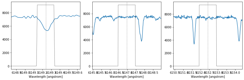
The FeII index lines are added in the bottom. Now, the FeII index can be used by calling I_FeII in the option indices inside ACTIN, if the new modified table is given as an input using the table_df option. The FeII lines can be plotted easily:

import os, glob
file = glob.glob(os.path.join(os.pardir, "actin2", "test", "HARPS-N", "*_s1d_A.fits"))

%matplotlib inline
actin.plot_index_lines(file, 'I_FeII', table_df=ind_tab.table)

And the index calculated:

df = actin.run(file, "I_FeII", table_df=ind_tab.table, progress=False)
df[['I_FeII', 'I_FeII_err']]

	I_FeII	I_FeII_err
0	0.451275	0.001272

If you are testing new indices it could be useful to also extract the individual fluxes in the lines. This can be done by activating the full_output option via the calcind_kw keyword argument:

df = actin.run(file, "I_FeII", table_df=ind_tab.table, calcind_kw=dict(full_output=True), progress=False)
df[['FeII_F', 'FeII_F_err', 'FeIIR1_F', 'FeIIR1_F_err', 'FeIIR2_F', 'FeIIR2_F_err']]

	FeII_F	FeII_F_err	FeIIR1_F	FeIIR1_F_err	FeIIR2_F	FeIIR2_F_err
0	686190.952148	1852.282959	763766.467285	873.937326	756793.547852	869.938783